

.jpg)
Passionate about forward osmosis technologies and their commercial applications & adaptations.
- Forward osmosis is not dead – interview with leading water consultant Walid Khoury - August 30, 2020
- Listing of major commercial & academic FO players on ForwardOsmosisTech - April 12, 2020
- 0.26MGD FO-SWRO Hybrid for seawater desalination achieves 25% energy reduction compared to MF/SWRO - December 14, 2019
What is concentration polarization and why does it limit forward osmosis membrane performance?
Concentration polarization is the build-up of concentration gradients both inside and around forward osmosis membranes during operation. Said gradients reduce the effective osmotic pressure difference across the membrane active layer and thus limit the attainable water flux.
In membrane processes there are – generally speaking – 4 types of concentration polarization falling into two main categories, namely external concentration polarization (ECP) and internal concentration polarization (ICP), and two sub-categories; dilutive and concentrative:
For dense, symmetric membranes that reject feed and draw solutes, external concentration polarization takes places at the membrane surfaces:
- On the feed side, solutes are concentrated at the surface, as water permeates through the membrane, giving rise to concentrative ECP
- On the draw side, solutes are diluted at the surface, as water enters from the feed side, giving rise to dilutive ECP
For asymmetric membranes – containing both a dense rejection layer and an underlying porous support – internal concentration polarization takes place in the porous support layer and external concentration polarization on the inter-phase between the rejection layer and surrounding solutions:
- When the dense rejection layer faces the feed solution (known as AL-FS or “FO-mode” configurations), the water permeating through the porous support layer dilutes the draw solutes inside the support, giving rise to dilutive ICP. In addition, concentrative ECP takes place on the dense rejection layer
- When the dense rejection layer faces the draw solution (known as AL-DS or “PRO-mode” configurations), solutes inside the support are concentrated as water permeates through the membrane, giving rise to concentrative ICP. In addition, dilutive ECP takes place on the dense rejection layer
Having introduced the basic concepts, the next part of this article will present a detailed overview of concentration polarization effects in FO membranes from a more scientific point of view. Equations, data and figures are based – among others – on the excellent research article by McCutcheon et. al.:
“Influence of concentrative and dilutive internal concentration polarization on flux behaviour in forward osmosis”, McCutcheon et. al. 2006
Forward osmosis membrane performance parameters and equations
In forward osmosis processes, the water flux Jw across the membrane and the reverse salt flux Js from draw to feed are important membrane performance parameters. Jw and Js are determined by the following equations:
Jw = AΔ∏e
- A is the “pure water permeability coefficient” – an intrinsic membrane property
- Δ∏e is the effective osmotic pressure difference across the membrane’s active layer (the dense rejection layer)
- Jw is predominantly reported in L/m2h or LMH in short
Js = BΔC
- B is the “salt permeability coefficient” – an intrinsic membrane property depending on the solutes used in the draw solution
- ΔC is the difference in solute concentration across the active layer
- Js is predominantly reported in g/m2h or GMH in short
Thus, the build-up of concentration gradients in concentration polarization phenomena reduce both Jw and Js through a decrease in both the effective osmotic pressure difference and the difference in solute concentration across the active layer, respectively. In order to quantify concentration polarization effects, the following assumption is traditionally made (McCutcheon et. al., 2006):
- Js does not affect bulk solute concentrations and is therefore not considered
With this assumptions in place, the effective osmotic pressure across a FO membrane experiencing concentration polarization becomes (McCutcheon et. al., 2006):
AL-FS configuration: dilutive ICP & concentrative ECP
Δ∏e = ∏D,m – ∏F,m = ∏D,B*exp(-JwK) – ∏F,B*exp(Jw/k)
- ∏D,m is the osmotic pressure of the draw solution on the draw side of the active layer
- ∏F,m is the osmotic pressure of the feed solution on the feed side of the active layer
- ∏F,B is the bulk osmotic pressure of the feed solution
- ∏D,B is the bulk osmotic pressure of the draw solution
- Jw is the water flux
- K is the solute resistivity for diffusion (see below)
- k is the mass transfer coefficient
- exp(-JwK) is the reduction factor of draw solution osmotic pressure due to dilutive ICP
- exp(Jw/k) is the amplification factor of feed solution osmotic pressure due to concentrative ECP
In the case of feed solutions with low bulk osmotic pressures, the effect of concentrative ECP is limited meaning that ∏F,m ≈ ∏F,B (i.e. exp(Jw/k) = 1). Hence, in forward osmosis processes under the AL-FS configuration, the main contribution to concentration polarization comes from dilutive ICP when the feed water has low osmotic pressure.
AL-DS configuration: concentrative ICP & dilutive ECP
Δ∏e = ∏D,m – ∏F,m = ∏D,B*exp(-Jw/k) – ∏F,B*exp(JwK)
- exp(-Jw/k) is the reduction factor of draw solution osmotic pressure due to dilutive ECP
- exp(JwK) is the amplification factor of feed solution osmotic pressure due to concentrative ICP
- See above for remaining parameter descriptions
In the case of feed solutions with low bulk osmotic pressures, the effect of concentrative ICP is limited meaning that ∏F,m ≈ ∏F,B (i.e. exp(JwK) = 1). Hence, in forward osmosis processes under the AL-DS configuration, the main contribution to concentration polarization comes from dilutive ECP when the feed water has low osmotic pressure.
The mass transfer coefficient k depends on the flow configuration across membrane surfaces, which again is determined by characteristic dimensions of the flow chamber surrounding the FO membrane. Mass transfer coefficients are thus not determined by intrinsic FO membrane parameters and will not be treated in detail here. The solute resistivity for diffusion (K) turns out to be a key determinant of FO membrane performance determined – in part – by intrinsic membrane parameters . Within the scientific field of FO membrane performance optimization, the majority of developments are focused on reducing K values. And from the equations above it is easy to see why.
The smaller the K value, the easier it is for solutes to diffuse inside the porous support layer, and the smaller the negative effect of internal concentration polarization on membrane performance becomes.
The K value therefore deserves further elaboration:
K = (t*τ)/(D*ε) = S/D , where S = (t*τ)/(ε)
- t is the support layer thickness
- τ is the support layer tortuosity (a measure of the degree of “twisting” of the pores in the support layer)
- ε is the support layer porosity (a measure of the amount of “empty” space in the support layer)
- D is the diffusion coefficient of the draw solute
- S is known as the structural parameter and it is an intrinsic property of the support layer. Typical S values for good forward osmosis membranes are around 300μm (Tiraferri et. al., 2011)
For a great article relating performance of FO membranes to the structural parameters of their support layers, please refer to:
“Relating performance of thin-film composite forward osmosis membranes to support layer formation and structure”, Tiraferri et. al. 2011
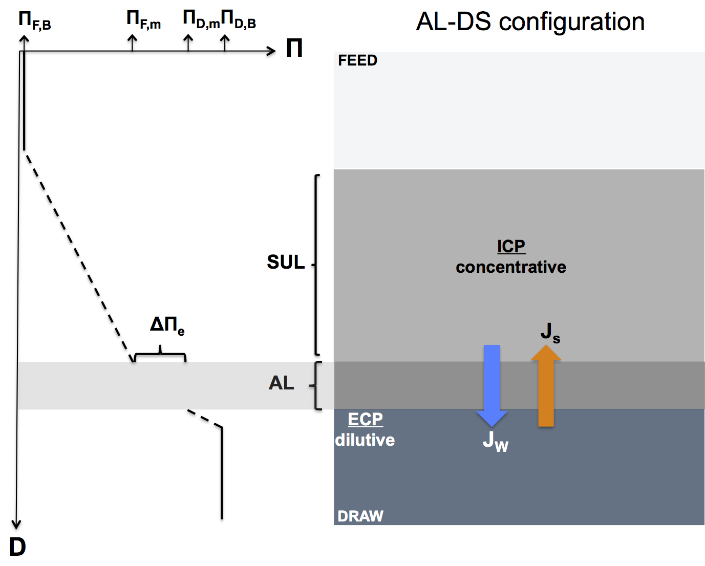
Forward osmosis concentration polarization when the active layer faces the draw solution (AL-DS or “PRO mode” configuration)
The figure below illustrates how concentration polarization reduces the effective osmotic driving force in the AL-DS configuration. Notice that both external and internal concentration polarization have been included in the figure for illustrative purposes.
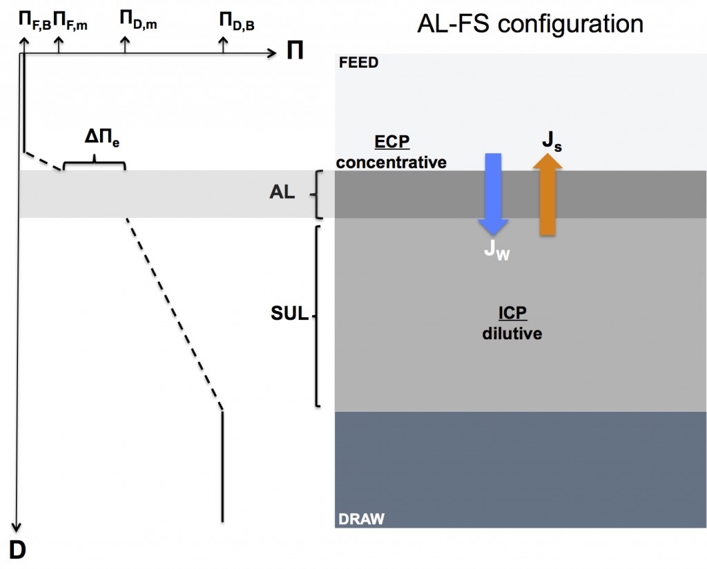
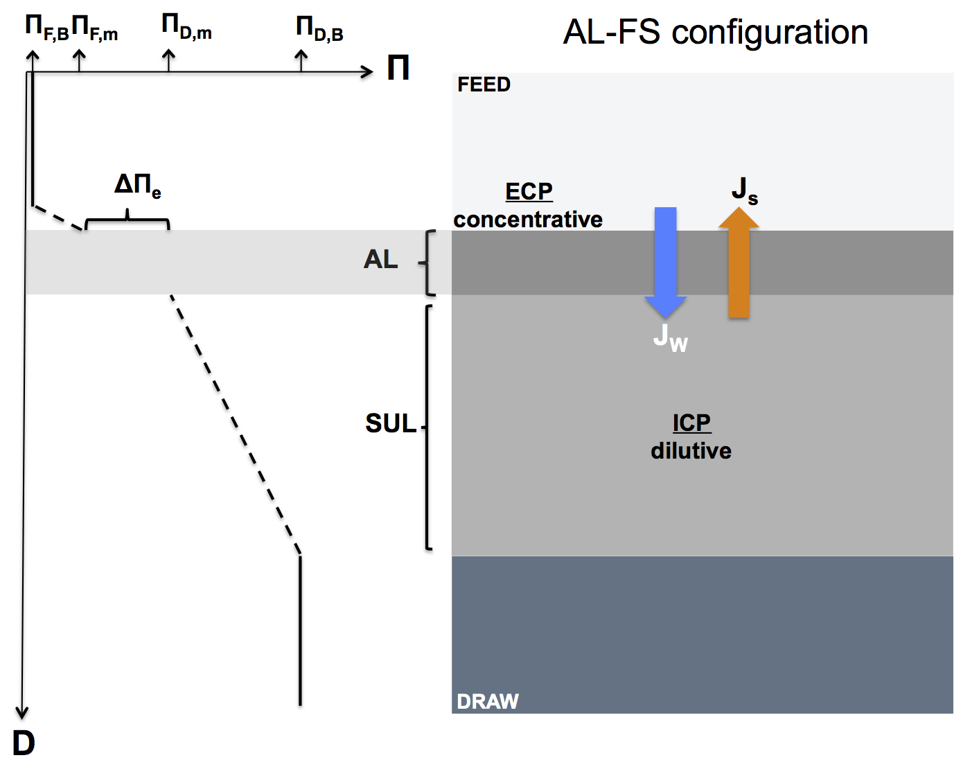
Forward osmosis concentration polarization when the active layer faces the feed solution (AL-FS or “FO mode” configuration)
The figure below illustrates how concentration polarization reduces the effective osmotic driving force in the AL-FS configuration. Notice that both external and internal concentration polarization have been included in the figure for illustrative purposes.
Some calculated examples of flux reduction as a result of internal concentration polarization
The numbers in the tables below are based on the following data for a good performing forward osmosis membrane with sodium chloride (NaCl) as draw solution:
- S = 300μm (Tiaferri et. al., 2011)
- DNaCl = 1,61*10-9 m2/s (Philip et. al., 2010)
- A = 2 LMH/bar (Tiaferri et. al., 2011)
→Let’s first examine the case where there’s no internal concentration polarization:
| ∏D,B (bar) | ∏F,B (bar) | Δ∏ (bar) | Jw (LMH) |
| 20 | 4 | 16 | 32 |
| 30 | 4 | 26 | 52 |
| 40 | 4 | 36 | 72 |
| 50 | 4 | 46 | 92 |
→And the case with concentrative ICP in the AL-DS configuration:
| ∏D,B (bar) | ∏F,B (bar) | Fixed Jw (LMH) | Fixed Jw (m/h) | Jw*K | ∏F,m (bar) | Δ∏e (bar) | Jw potential (LMH) |
| 20 | 4 | 10 | 0,01 | 0,52 | 7 | 13 | 26 |
| 30 | 4 | 20 | 0,02 | 1,0 | 11 | 19 | 38 |
| 40 | 4 | 30 | 0,03 | 1,6 | 19 | 21 | 42 |
| 50 | 4 | 40 | 0,04 | 2,1 | 32 | 18 | 36 |
In the calculations above, a fixed system water flux has been adopted and based on this value, the reduced osmotic pressure difference (Δ∏e) due to concentrative ICP has been calculated along with the water flux potential associated with the reduced osmotic pressure difference. Now, fixing the system water flux is a bit artificial – but a necessary step to performing the calculations. It is interesting to note, that Δ∏e for the ∏D,B = 50 example is actually lower than for ∏D,B = 40, indicating that progressively higher draw solution osmotic pressures are needed to overcome concentration polarization effects in high-flux FO processes. This fact is illustrated in the following table where it has been calculated what the bulk draw solution bulk osmotic pressures should actually be for the fixed Jw‘s to equal the potential Jw‘s.
| ∏D,B, actual (bar) | ∏F,B (bar) | Fixed Jw (LMH) | Fixed Jw (m/h) | Jw*K | ∏F,m (bar) | Δ∏e (bar) | Jw potential (LMH) |
| 12 | 4 | 10 | 0,01 | 0,52 | 7 | 5 | 10 |
| 21 | 4 | 20 | 0,02 | 1,0 | 11 | 10 | 20 |
| 34 | 4 | 30 | 0,03 | 1,6 | 19 | 15 | 30 |
| 52 | 4 | 40 | 0,04 | 2,1 | 32 | 20 | 40 |
→And finally, the same two tables for dilutive ICP in the AL-FS configuration:
| ∏D,B (bar) | ∏F,B (bar) | Fixed Jw (LMH) | Fixed Jw (m/h) | Jw*K | ∏D,m (bar) | Δ∏e (bar) | Jw potential (LMH) |
| 20 | 4 | 10 | 0,01 | 0,52 | 12 | 8 | 16 |
| 30 | 4 | 20 | 0,02 | 1,0 | 11 | 7 | 14 |
| 40 | 4 | 30 | 0,03 | 1,6 | 8 | 4 | 8 |
| 50 | 4 | 40 | 0,04 | 2,1 | 6 | 2 | 4 |
| ∏D,B, actual (bar) | ∏F,B (bar) | Fixed Jw (LMH) | Fixed Jw (m/h) | Jw*K | ∏D,m (bar) | Δ∏e (bar) | Jw potential (LMH) |
| 15 | 4 | 10 | 0,01 | 0,52 | 9 | 5 | 10 |
| 39 | 4 | 20 | 0,02 | 1,0 | 14 | 10 | 20 |
| 90 | 4 | 30 | 0,03 | 1,6 | 19 | 15 | 30 |
| 190 | 4 | 40 | 0,04 | 2,1 | 24 | 20 | 40 |
Notice how the draw solution osmotic concentration must be increased to 190 bar to achieve a Jw of 40 LMH in the AL-FS configuration whereas only 52 bar was necessary to achieve the same flux in the AL-DS configuration. This example clearly demonstrates how dilutive internal concentration polarization on the draw side has a severer negative effect on water flux than concentrative internal concentration polarization on the feed side. For the same reason, researchers, publishing articles on forward osmosis membrane developments, almost always choose the AL-DS configuration when determining membrane water flux performance:
Membrane researchers prefer the AL-DS when reporting the performance of their membranes, because forward osmosis membranes have the best water flux performance in this configuration
Notes: We do our best to check the validity of our calculations, however, no responsibility is taken for calculation errors.